Boundary conditions for bars

Which internal forces can be transferred (or which rigidity a connection) between the ends of two bars, is determined using this button .
The following dialogue appears:

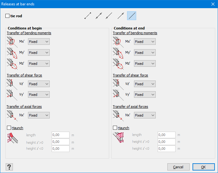
You see quick buttons (see further) and two columns to define the boundary conditions at the start and end point of bar.

• Start point = point with the smallest X-coordinate
  • If X-coordinates are the same, it’s the point with the smallest Y-coordinate
    • If Y-coordinates are the same, it’s the point with the smallest Z-coordinate
• End point = the other point

This dialog can contain padlocks depending on the properties of the elements you have selected. Read all about the padlocks in this article.

Top part (quick buttons)

The meaning of the quick buttons is as follows:

• : tie rod
  A bar in which only axial tension can be transferred. The use of tie rods always results in an iterative calculation due to their non-linear behaviour.
  The quick buttons for tie rods sometimes give iterations problems in the elastic analysis. The solution is then to model the tie rods using a function instead of using the quick buttons.
  
  A tie rod is not the same as a cable. A cable (= like a clothes line) cannot be modelled in Diamonds (more info).
  
  The counter part of a tie rod is a compression bar.
• : hinged bar
  At both bar ends My’ and Mz’ cannot be transferred. All other forces can be transferred.
• : hinge at the start of the bar
  At the start point of the bar My’ and Mz’ cannot be transferred. All other forces can be transferred.
• : hinge at the end of the bar
  At the end point of the bar My’ and Mz’ cannot be transferred. All other forces can be transferred.
• : clear all hings
  At both bar ends, all internal forces can be transferred

Whenever you select a quickbutton, the relevant options will be turned on/off in the middle of the dialog.

Middle part

Instead of using the quick buttons, you can restrict the various degrees of freedom directly. For each degree of freedom, using the pull-down menu, you can:

• set the degree of freedom fixed.
• enter a spring using a value.
• enter a function (see below).

Custom function

A rigidity diagram presents the displacement (or angular displacement) in relation to the applied force (reaction force, moment, normal force or shear force). The definition of a rigidity diagram is at the end of a bar is similar to the definition for a support.

• Select the option “Function” from the drop down menu.
• Either choose one of the existing functions or define a new one using .
  A new dialogue appears.
• Click .
  
• Name the function.
• For each sign of the internal force, choose if:
  • the internal force cannot be transferred = free
  • the internal force can be transferred = fixed
  • the internal force can be transferred linear = value
  • the internal force can be transferred variable = function
    When you choose this option, keep the following remarks in mind:
    • The function must always go through the origin.
    • Avoid (almost) perfect horizontal or vertical branches in the graph.
      They describe a relation, not a function y= f(x). One x-value can lead to multiple solutions y or multiple x-values lead to the same solution. This causes arithmetic problems.
      Use gently sloping branches instead.
• You can save a defined function in a TXT-file using the button . An existing function (TXT format) can be loaded via .

Example of a custom function on a bar end	Example of a custom function on a support
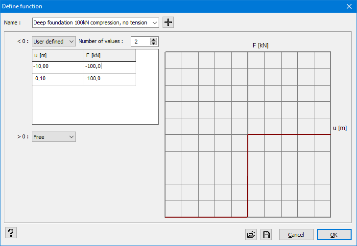The diagram shows that the rotation rigidity M/φ is constant as long as the applied moment is less than 45,4kNm. Once the moment is exceeded, the rigidity varies according to M. If the moment exceeds 68,2kNm, a plastic hinge is formed because an additional moment produces an angular deformation infinitely large.	The foundation can’t bear tension and only 100kN compression. The rigidity diagram should lay in the 1st and 3rd quadrant because in the formula F=k∙x the spring constant k cannot take on a negative value. If the function does not have a valid range, a red message will appear below this window.

Bottom part (haunch)

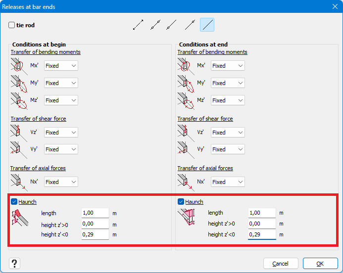
• You can add haunches at the the begin and/or end point of the selected bars.
  Check the box(es) before the relevant options.
• Enter the length of the haunch.
  A haunch usually starts at the length of 1m.
• Enter the height of the haunch.
  A good starting point is to set the height haunch equal to the height of the beam above. For example: a haunch below an IPE 300 gets a height of 0,29m.
  
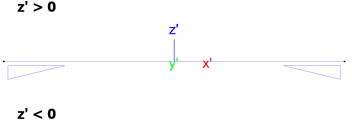
  “Height z’ < 0” refers to the lower side of the beam. And “Height z’ > 0” refer to the upper side of the beam.
  
  z’ is local coordinate system of the beam. It can be shown on the screen using the Configuration settings .

How are haunches taken into account in the calculations?

• The cross-section of the haunch equals the cross-section of the beam above it, minus the top flange.
  It is not possibel to change the cross-section of the haunch in Diamonds. That’s only possible in PowerConnect (see further).
• A haunch will locally increase the stiffness of the cross section (moment of interia) for the global analysis .
• The position of the bolts, end plate, welds, … are irrelevant for Diamonds. Same for a detailed choice of the cross-section of the haunch. The purpose of a haunch in Diamonds is to calculate with the additional stiffness that results from the haunch. Not to perform a detailed calculation of the connection itself.
  
  Once the structure is designed (= sufficient for strenght, stability and stiffness), you can send the connection to PowerConnect. In PowerConnect you can adjust the cross-section, bolts, end plate, … If you change the cross-section of the haunch in PowerConnect, send the connection back to Diamonds, the global analysis in Diamonds, will be made with the adjusted cross-section.