DLD 02: Mass-spring system with 2 degrees of freedom – modal information

Description

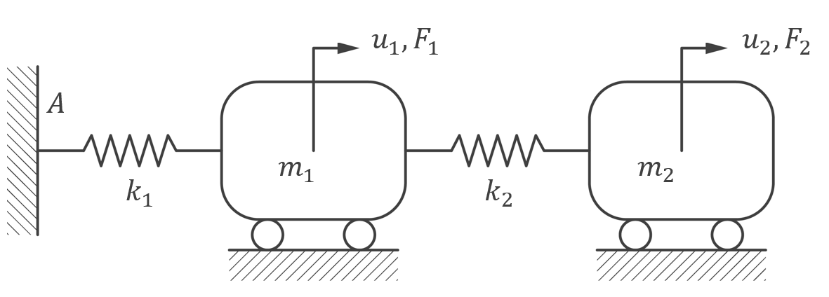
Geometry	Mass	$m_1=50kg$ $m_2=80kg$
	Spring contant	$k_1=4000N/m$ $k_2=6000N/m$
	Damping ratio’s	$\xi=0.02$ $\xi=0.05$
Mesh	No. of divisions	1

The damping ratio’s are imposed in the dialog for modal analysis .

Independent reference results

Open hand calculations

In this example we want to recalculate the modal information. To do so, we’ll be using the same model as in DLD 01.
The modal information can be found after this button . Make sure to check the option « Display all the information« .

Natural frequencies $f$

These are the specific rates at which a system naturally vibrates, determined solely by its mass and stiffness distribution. This data was already available in the validation example DLD 01.

$f=\begin{bmatrix} 0.778 \\ 2.522 \end{bmatrix} \text{[Hz]}$

Angular frequencies $\omega$

The relation between the angular frequencies and the natural frequencies is given by:

$\omega = 2 \pi f=2 \pi \begin{bmatrix} 0.778 \\ 2.522 \end{bmatrix} = \begin{bmatrix} 4.888 \\ 15.845 \end{bmatrix} \text{[1/s]}$

Natural periods $T$

The relation between the natural period and the natural frequency is given by:

$T= 1/ f= \begin{bmatrix} 0.778 \\ 2.522 \end{bmatrix} = \begin{bmatrix} 1.285\\ 0.397 \end{bmatrix} \text{[s]}$

Modal mass $M$

The shape modes were calculated in DLD 01. The first column represents the displacements of mode 1, and the second of mode 2.

$\phi=\begin{bmatrix} 67.036774& 124.441490\\ 98.379631& -52.997219 \end{bmatrix}$

The modal mass $M$ is calculated as:

$M=\phi^{T} \cdot M_m \cdot \phi=\begin{bmatrix} 10^6 & 0\\ 0 & 10^6 \end{bmatrix} \text{kg}$

$M_m$ is the mass matrix $M_m=\begin{bmatrix} 50 &0 \\ 0& 80 \end{bmatrix} \text{kg}$ .

In the Diamonds results for the modal mass $M$ , the $10^6 kg$ is left out. You just see « 1 » in the table. The mass matrix $M_m$ cannot be consulted in Diamonds.

Modal stiffness $K$

The modal stiffness $K$ can be calculated in two ways resulting in the same result:

$K=M \cdot \omega^2=\begin{bmatrix} 23.870 \\ 250.850 \end{bmatrix} \frac{kN}{mm}$

$K=\phi^T \cdot K_k \cdot \phi=\begin{bmatrix} 23.870 &0 \\ 0& 250.850 \end{bmatrix} \frac{kN}{mm}$

$K_k$ is the stiffness matrix $K_k=\begin{bmatrix} k_1+k_2 & -k_2 \\ -k_2 & k_2 \end{bmatrix}=\begin{bmatrix} 10000 & -6000 \\ -6000 & 6000 \end{bmatrix} \frac{N}{m}$ .

The stiffness matrix $K_k$ cannot be consulted in Diamonds.

Modal damping $D$

Rayleigh damping was used in this model. In order to calculate the modal damping $D$ , we should calculate the damping matrix $D_d$ first.

$a_0=\frac{2 \cdot \omega_1 \cdot \omega_2 \cdot \left( \xi_2 \cdot \omega_1 - \xi_1 \cdot\omega_2 \right)}{\omega_1^2-\omega_1^2}=0.05 \frac{1}{s}$

$a_1=\frac{2 \cdot \left( \xi_1 \cdot \omega_1 - \xi_2 \cdot\omega_2 \right)}{\omega_1^2-\omega_1^2}=6.11 \cdot 10^{-3} \text{s}$

The damping matrix $D_d$ becomes:

$D_d=a_0\cdot M_m + a_1 \cdot K_k=\begin{bmatrix} 63.61 & -36.68 \\ -36/68 & 40.64 \end{bmatrix} \frac{kg}{s}$

The damping matrix $D_d$ cannot be consulted in Diamonds. But using the damping matrix $D_d$ we can calculate the modal damping $D$ :

$D=\phi^T \cdot D_d \cdot \phi=\begin{bmatrix} 0.195 & 0\\ 0 & 1.583 \end{bmatrix} \frac{kN \cdot s}{mm}$

Critical damping $D_c$

Again using the damping matrix $D_d$ we can caluculate the critical damping $D_c$ :

$D_c=2 \cdot \sqrt{M \cdot K} = \begin{bmatrix} 9.776 \\ 31.660 \end{bmatrix} \frac{kN \cdot s}{mm}$

Damping ratio’s $\xi$

Since this model only has 2 DOF’s, there are only 2 damping ratio’s. If your model contains more DOF, the damping ratio’s of mode 3 until i can be calculated using:

$\xi_i=\frac{1}{2}\left( \frac{a_0}{2\pi f_i} +a_1 \cdot 2\pi f_i\right)$

Ratio of the effective modal mass in a mode to the total mass

To calculate this ratio we need the modal participation factor $\gamma$ . The modal participation factor $\gamma$ cannot be consulted in Diamonds.

$\gamma=\phi^T \cdot M_m \cdot \begin{bmatrix} 10^{-3}\\ 10^{-3} \end{bmatrix}=\begin{bmatrix} 11.222 \\ 1.982 \end{bmatrix} \text{kg}$

From the modal participation factor $\gamma$ we can determine the effective modal mass $m_eff$ . The effective modal mass $m_eff$ cannot be consulted in Diamonds.

$m_{eff}=\frac{\gamma^2}{1 \text{kg}}=\begin{bmatrix} 125.94 \\ 3.93 \end{bmatrix} \text{kg}$

Note that the sum of 125.94 + 3 .93 = 129.87kg which equals the sum of the masses in the system 50+80kg = 130kg.

Now let’s calculate the ratio of the effective modal mass to the total mass for each mode. It’s this ratio that you see in Diamonds.

$\frac{m_{eff}}{130kg}=\begin{bmatrix} 96.88\\ 3.02 \end{bmatrix}$ %

Results

	Independent reference	Diamonds	Difference¹
$f$ [Hz]	0.778 2.522	0.778 2.522	≈0.00%
$\omega$ [1/s]	4.888 15.845	4.886 15.837	≈0.00%
$T$ [s]	1.285 0.397	1.286 0.397	≈0.00%
$M$	1 1	1 1	≈0.00%
$K$	23.870 250.850	23.869 250.812	≈0.00%
$D$	0.195 1.583	0.195 1.584	≈0.00%
$D_c$	9.776 31.660	9.771 31.674	≈0.00%
$\frac{m_{eff}}{m_{tot}}$	96.88% 3.02%	96.97% 3.03%	≈0.00%

References

Hofman, G. E. (2012). Eindige Elementen Methode: Deel 2. MERc, p118

Tested in Diamonds 2026.

Article Attachments

.bsf

DLD 01 196 Ko

Was this article helpful?

Yes No

Need Support?

Can't find the answer you're looking for? Don't worry we're here to help!

CONTACT SUPPORT

Description

Independent reference results

Natural frequencies

Angular frequencies

Natural periods

Modal mass

Modal stiffness

Modal damping

Critical damping

Damping ratio’s